


In my previous blog post I talked about how to get Twitter data into Power BI. This article will discuss how you can apply text mining on that data with some R code, together with some Power BI visuals. At the end of the article we will have made an interactive word cloud with the frequency of words.
In case you don’t know how to get twitter data into Power BI, then I would like to refer to my previous post.
So last time our R script stopped with our data frame df_tweets. For text mining, however, we first need to clean up all our tweets. We don’t need:
Stop words are words which do not contain important significance, like a, and, in, etc, I, … We will also be including the word powerbi on itself since it doesn’t give extra meaning to our data. Let’s look at the code:
[html]#copy column
df_tweets$cleansedText <- df_tweets$text

#remove graphical characters
df_tweets$cleansedText <- str_replace_all(df_tweets$cleansedText,"[^[:graph:]]", " ")

#convert tweet to lower
df_tweets$cleansedText <-tolower(df_tweets$cleansedText)

# Remove RT
df_tweets$cleansedText <- gsub("\\brt\\b", "", df_tweets$cleansedText)

# Remove usernames
df_tweets$cleansedText <- gsub("@\\w+", "", df_tweets$cleansedText)

# Remove punctuation
df_tweets$cleansedText <- gsub("[[:punct:]]", "", df_tweets$cleansedText)

# Remove links
df_tweets$cleansedText <- gsub("http\\w+", "", df_tweets$cleansedText)

# Remove tabs
df_tweets$cleansedText <- gsub("[ |\t]{2,}", "", df_tweets$cleansedText)

# Remove blank spaces at the beginning
df_tweets$cleansedText <- gsub("^ ", "", df_tweets$cleansedText)

# Remove blank spaces at the end
df_tweets$cleansedText <- gsub(" $", "", df_tweets$cleansedText)[/html]
The first line of the code makes a new column cleansedText in our data frame, a copy of our twitter messages. That way we will do a clean up on a copy, and keep the original, which might be useful later. In the next lines everything is converted to lower case, removing RT (retweet), usernames, punctuation, links, tabs and blank spaces. All this is done with the gsub() function, a default R function for text replacement and Regex.
The following tweet: The latest The #PowerBI Daily! https://t.co/2ZCFOhO288 #powerbi #bi would become the latest the powerbi dailypowerbi bi. The last ast clean-up step is removing stop words. To do this, we need to convert our data frame to a corpus. A corpus is a specific class that can be identified as a library of documents, or in our example, tweets, which belongs to the tm package within R.
[html]# Create Corpus
tweet_corpus <- Corpus(VectorSource(df_tweets$cleansedText))

# Removing Stop Words
tweet_corpus <- tm_map(tweet_corpus, function(x)removeWords(x,c(stopwords("english"), search_term)))[/html]
Now that our data is cleansed, a Term Document Matrix (TDM) is necessary. A TDM is a matrix in which the rows contain all the words that are used in each document (tweet) and in which the columns contain the documents (tweets).
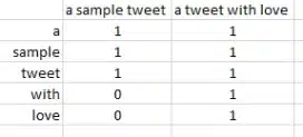
An example TDM
[html]tweet_tdm <- TermDocumentMatrix(tweet_corpus)[/html]
As you can imagine, depending on how much text you are analysing, this TDM could become pretty big. What we would like to do is get a word cloud in Power BI that shows us the most common words. We aggregate our TDM, group it by word and remove the details of the tweet. By converting it to a matrix, we can aggregate with the rowSums() function and then sort descending on the frequency of the word.
[html]tweet_tdm_m <- as.matrix(tweet_tdm)
tweet_tdm_m <- sort(rowSums(tweet_tdm_m),decreasing = TRUE)[/html]
Again depending on your tweets or documents, this may give you a matrix with thousands of words. For our report we only want the top 150. You can do this by creating a new data frame and then only keeping the top 150. As last step in this code, I added a WordId and filled it with a sequence number. I did this because I would like to link the words back to the tweets. That way I will be able to click a certain word in my Power BI report and then see the tweets.
[html]df_tweets$TweetId<-seq.int(nrow(df_tweets))[/html]
The last step is to create a mapping table between the Tweets and the Words. The function grep() is executed on each word, looking up which tweet makes use of a certain word and then saves this data. At the end, we have a data frame with two columns TweetId and WordId.
[html]#Tweet_Word_Mapping
list_tweet_word_map <- sapply(1:nrow(df_wordcount_top), function(x) grep(df_wordcount_top[x,"keyName"], df_tweets$cleansedText))
word_map_names <- c("TweetId","WordId")
df_tweet_word_map <- NULL
for(x in 1:nrow(df_wordcount_top)){
  df_tweet_word_map <- rbind(df_tweet_word_map, setNames(data.frame(list_tweet_word_map[x], x), word_map_names))
}
df_tweet_word_map <- df_tweet_word_map[,word_map_names][/html]
Now let’s load all of this in Power BI and make a nice report!
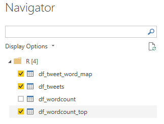
Your data is loaded! By default, Power BI does not have a WordCloud visual, but in the Custom Visual Gallery there is one you can download and use. Discover here how you can use a custom visual.
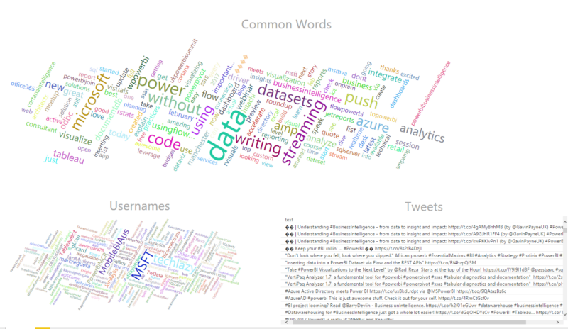
I’m not going to go through the whole process of making the Power BI report here, but I did make a small video on how I did it and what it looks like.
This was a small introduction into Text mining with R and visualising it in Power BI. Of course, you can immediately make your visuals in R too, but then you don’t have the interactivity with the other visuals in your report.
Our final report:

Crafted by ![]()
Crafted by ![]()


